Neurophysioloy and Neural Nets

This is an evaluated Mathematica notebook. Since the notebook is intended to be interactive, it may be helpful to also view the unevaluated version

MA 354 - Mathematical Modeling

Richard Hitt

Introduction

We will take a brief look at different ways to approach mathematical modeling of animal nervous systems. First, we will look at the famous model of the neuron due to Hodgkin and Huxley. Through several brilliantly crafted experiments in the early 1950s, they discovered the basic mechanisms of sodium and potassium in the creation of action potentials in neurons. We will see that their four-variable system of differential equations accurately simulates an action potential in a neuron.

After we understand the basic physiology of the neuron, we can look at ways to model networks of neurons. We will build a simple nervous system which simulates perception of heat and cold. It will also simulate the parlor trick in which a blindfolded person briefly touches a very cold object and reports a sensation of heat.

Some Biology

The following picture show the basic anatomical structure of a neuron.

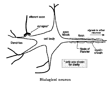
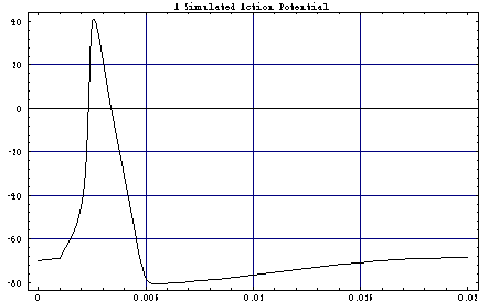
Neurotransmitters arrive at the depicted neuron from efferent axons. These neurotransmitters are either excitatory or inhibitory. The excitatory neurotransmitters tend to depolarize the neuron from its resting potential of around -70 millivolts. The inhibitory ones hyperpolarize the neuron. The cell body integrates all the depolarizing and hyperpolarizing impulses of the neurotransmitters. Once the electrical potential of the neuron falls above a threshold of around -40 or -50 millivolts, an action potential occurs. This action potential travels along the axon and results in the firing of a neurotransmitter at the end of the axon.

Chapter 8 of the Herod, Shonkwiler and Yeargers text explain in detail the mechanism involved in the creation of an action potential.

The Action Potential Model of Hodgkin-Huxley

The following notation will be explained in class and will be used to derive the four-variable system of differential equations used to simulate the action potential of a neuron. This material is explained in Chapter 8 of the preliminary version of "An Introduction to Mathematical Biology" by Herod, Shonkwiler and Yeargers.

In[1]:=

  Ena    = 55;
  Ek     = -82;
  El     = -59;
  gkbar  = 24.34;
  gnabar = 70.7;
  gl     = 0.3;
  vrest  = -70;
  Cm     = 0.001;
  alphan[v_] := 
    0.01*(10 - (v - vrest))/(Exp[0.1*(10 - (v - vrest))] - 1)
  betan[v_]  := 0.125*Exp[-(v - vrest)/80]
  alpham[v_] := 
    0.1*(25 - (v - vrest))/(Exp[0.1*(25 - (v - vrest))] - 1)
  betam[v_]  := 4*Exp[-(v - vrest)/18]
  alphah[v_] := 0.07*Exp[-0.05*(v - vrest)]
  betah[v_]  := 1/(Exp[0.1*(30 - (v - vrest))] + 1)
  pulse[t_]  := -10*(Sign[t - 0.001] - Sign[t - .002])

In[2]:=

  solution =
  NDSolve[
    { v'[t] == -(gnabar*m[t]^3*h[t]*(v[t] - Ena) +
                 gkbar*n[t]^4*(v[t] - Ek) + 
                 gl*(v[t] - El) + pulse[t])/Cm,
      n'[t] == 1000*(alphan[v[t]]*(1 - n[t]) - betan[v[t]]*n[t]),
      m'[t] == 1000*(alpham[v[t]]*(1 - m[t]) - betam[v[t]]*m[t]),
      h'[t] == 1000*(alphah[v[t]]*(1 - h[t]) - betah[v[t]]*h[t]),
      v[0]  == vrest,
      n[0]  == 0.315,
      m[0]  == 0.042,
      h[0]  == 0.608
    },
    {v[t],n[t],m[t],h[t]},
    {t,0,0.02},
    MaxSteps->1000
  ]

Out[2]=

  {{v[t] -> InterpolatingFunction[{0., 0.02}, <>][t], 
   
     n[t] -> InterpolatingFunction[{0., 0.02}, <>][t], 
   
     m[t] -> InterpolatingFunction[{0., 0.02}, <>][t], 
   
     h[t] -> InterpolatingFunction[{0., 0.02}, <>][t]}}

In[3]:=

  Plot[Evaluate[v[t] /. solution],
    {t,0,.02},
    GridLines->Automatic,
    Frame->True,
    PlotLabel->
      FontForm[
        "A Simulated Action Potential",{"Helvetica-Bold",20}
      ]
    ]

Out[4]=

  -Graphics-

McCulloch-Pitts (Discrete) Networks

Now that we have a rough idea of how a single neuron works, we can think about connecting several together to perform logical decisions. We will use a threhhold logic unit (TLU) to model the individual neurons. The TLU monitors its various inputs, summing their values. If the threshhold is reached, its fires a signal (represented by a real number) to the next TLU.

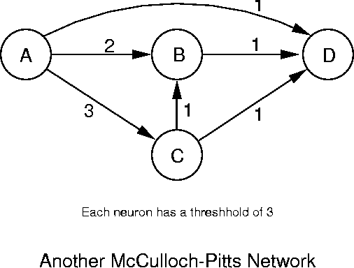
We will represent a neural network as a weighted, directed graph where the vertices are the neurons (TLUs), the edge weights are the values of the neurotransmitters, and the vertex weights are the threshhold values. For a first example, we c

[font = postscript; PICT; formatAsPICT; output; inactive; preserveAspect; pictureLeft = 0; pictureWidth = 450; pictureHeight = 353; pictureID = 131]

Continuous Networks

In real neurons, information is encoded in terms of frequency of transmission rather than merely the absence or presence of a transmission. Two modification are commonly made in the artificial neurons which have been developed so far in order to acommodate this. First, we can allow the inputs to be real numbers. We can do this either by postulating it, or by thinking of the numerical value as the frequency of the occurrences of pulses over a given fundamental unit of time. Also, we can make the frequency of output can be a continuous function of the depolarization of the neuron.

In[5]:=

  rho = 1;
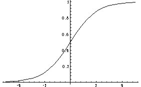
  Sigmoid[t_] := 1 / ( 1 + Exp[-t/rho])
  Plot[Sigmoid[t],{t,-5,5}]

Out[6]=

  -Graphics-

We can also view the threshhold of an individual neuron as a random variable with a Gaussian distribution. The probablility of the neuron firing then is the probablility that the potential is greater than this threshhold. The cumulative distribution

In[7]:=

  Plot[
    NIntegrate[
      (1/Sqrt[Pi])*Exp[-x^2],
      {x,-Infinity,t}
    ],
    {t,-5,5}
  ]

Out[8]=

  -Graphics-